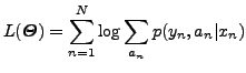
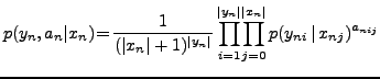
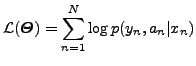
The so-called complete version of the log-likelihood
function (10) assumes that the hidden (missing) alignments
![]() are also known:
are also known:
The EM algorithm maximises (10) iteratively, through the
application of two basic steps in each iteration: the E(xpectation)
step and the M(aximisation) step. At iteration ![]() , the E step
computes the expected value of (12) given the observed
(incomplete) data,
, the E step
computes the expected value of (12) given the observed
(incomplete) data, ![]() , and a current estimation of
the parameters,
, and a current estimation of
the parameters,
![]() . This reduces to the computation
of the expected value of
. This reduces to the computation
of the expected value of ![]() :
:
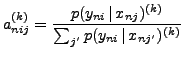
Then, the M step finds a new estimate of
![]() ,
,
![]() , by maximising (12),
using (13) instead of the missing
, by maximising (12),
using (13) instead of the missing ![]() . This
results in:
. This
results in:
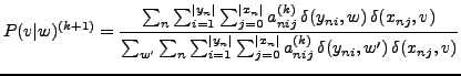 |
(14) |
for all
![]() and
and
![]() ; where
; where
![]() is the Kronecker delta function; i.e.,
is the Kronecker delta function; i.e.,
![]() if
if ![]() ; 0 otherwise.
; 0 otherwise.
An initial estimate for
![]() ,
,
![]() , is
required for the EM algorithm to start. This can be done by assuming that
the translation probabilities are uniformly distributed; i.e.,
, is
required for the EM algorithm to start. This can be done by assuming that
the translation probabilities are uniformly distributed; i.e.,
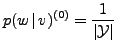 |
(16) |
![$\displaystyle = \frac{\sum_n \frac{p(w\,\vert\,v)^{(k)}}{\sum_{j'}p(w\,\vert\,x...
...um_{j=0}^{\vert x_n\vert} \,\delta(y_{ni}, w') \,\delta({x_{nj}, v)} \right ] }$](img52.png)